
In this analysis, we search for excited Ωb– states. The motivation and strategy for observing and measuring the masses and widths of these states is similar to that discussed here for the excited Ξb0 states search .
Evidence is sought by choosing a specific decay mode in which we expect such states to decay. An excited Ωb– state would have quark content bss. Consider the case, that a soft gluon is emitted from one of the quarks, and transforms into a uu pair. In the decay process, these 5 quarks could assemble as bsu + us, which could hadronize as Ξb0K–. If the gluon was to produce a dd pair, one could end up with a Ξb–K0. This mode is more difficult than the Ξb0K– mode because only about 35% of the K0 decays have a chance to be reconstructed in the Π+Π– final state. Taking into account the long lifetime of the KS0 meson, the detection efficiency is low, at least 10 times lower than reconstructing a single charged particle produced close to the collision point. Thus the most beneficial mode to search for excited Ωb– states is Ξb0K–.
Below, we show the topology for the decay of an excited Ωb– state, referred generically to as Ωb**-
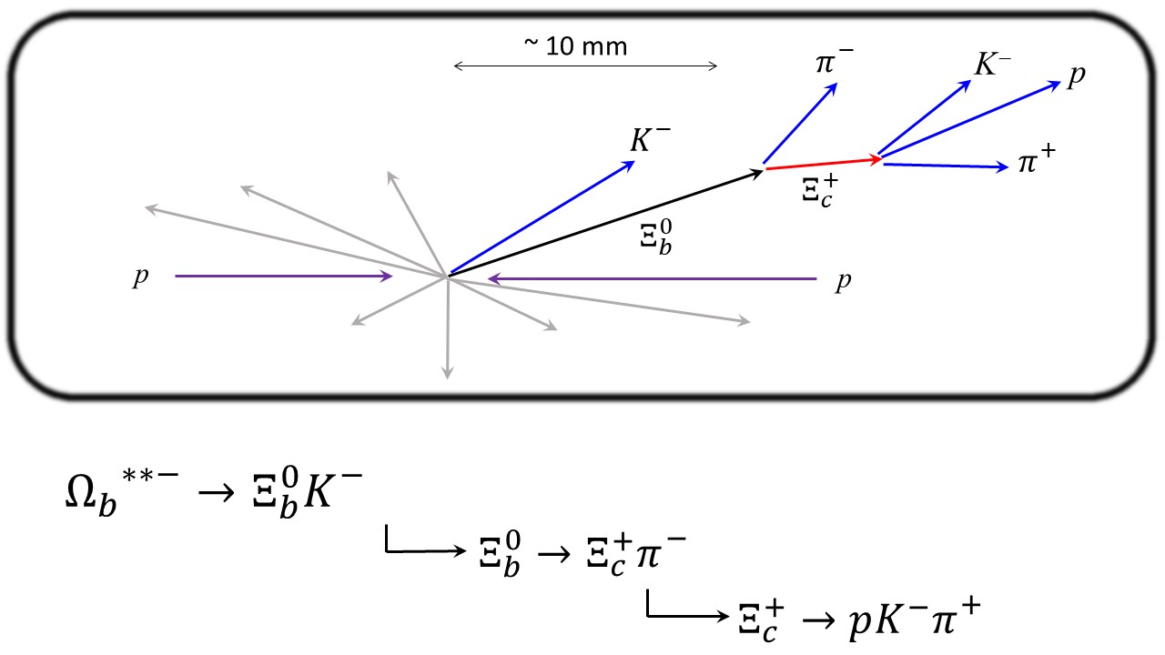
To reconstruct the Ωb– candidate, we “work backwards” in terms of the decay sequence. We first look to reconstruct a Ξc+ → p K–Π+ decay candidate. The p, K–, and Π+ particles are required to converge to a single point in 3D space (within the detector resolution), and have an invariant mass consistent with the known Ξc+ mass of 2468 MeV/c2. Then, this Ξc+ candidate is combined with a Π– meson to search for Ξb0 candidates. The Ξc+ Π– combination is required to have an invariant mass consistent with the known Ξb0 mass of 5792 MeV/c2. Exploiting the large Ξb0 lifetime of about ~1.5 ps (and ~0.45 ps for Ξc+), the p, K and Π decay products must be inconsistent with coming directly from the proton-proton collision point.. The invariant mass distribution of Ξc+Π– candidates passing all selection requirements is shown below. A prominent peak is seen at the expected Ξb0 mass. A fit to the data is overlaid.
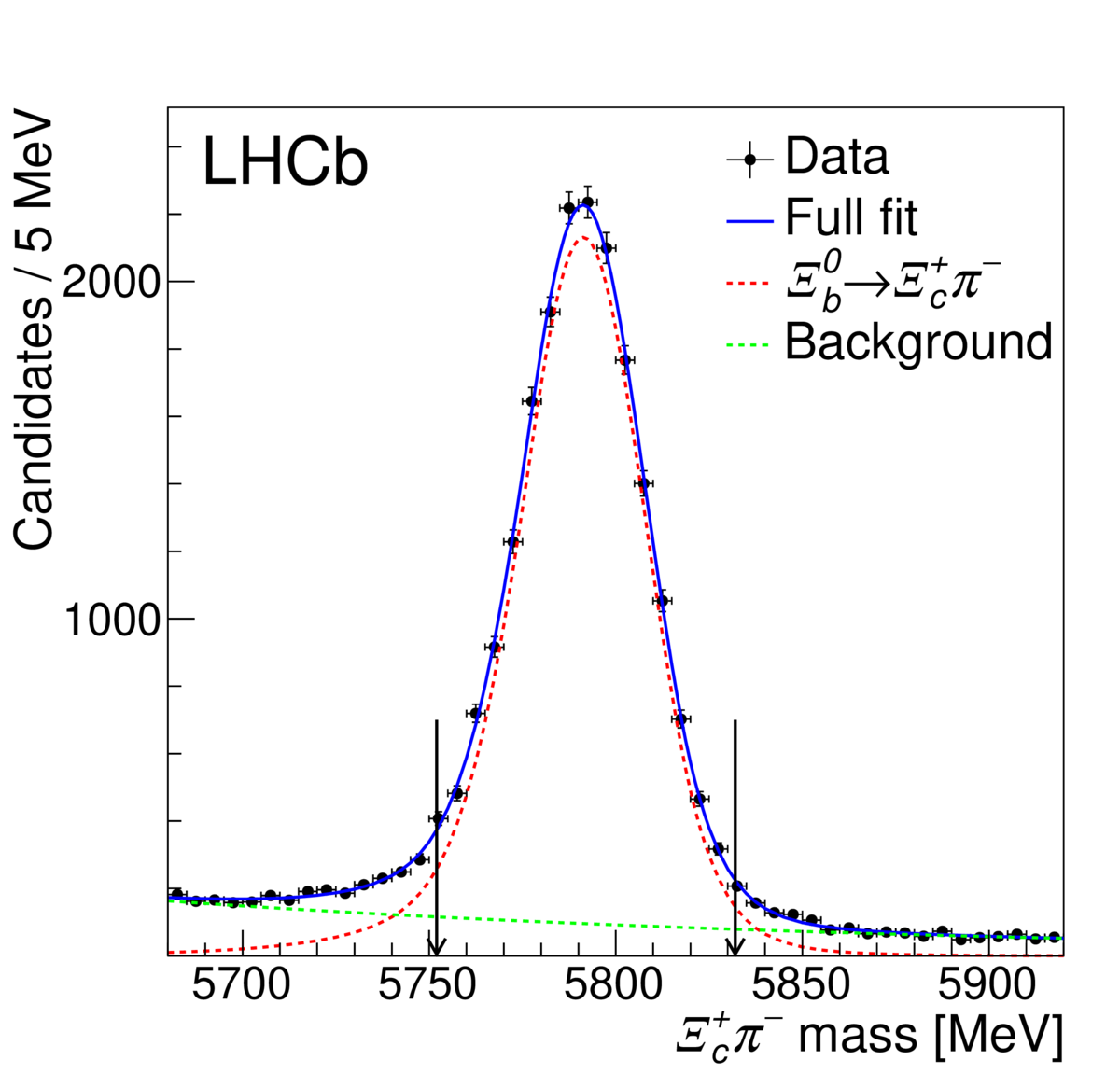
To search for the excited Ωb– states, a Ξb0 candidate (with a mass in between the arrows in the figure above) is combined with a K– meson that is consistent with coming from the pp interaction point. Here, the K– is taken from the pp interaction point because the decay is expected to be a strong decay, for which the decay time is immeasurably small, of order 10-23 sec.
Rather than use the invariant mass of the Ξb0K– candidate to search for the excited Ωb– state(s), we use the difference in invariant mass, M(Ξb0K–) – M(Ξb0), where in both cases, we are referring to the invariant mass of the decay products. The advantage of doing this is that the dominant component contributing to the mass resolution — namely that coming from the Ξb0 invariant mass determination — cancels in this difference. With this difference, the mass resolution is primarily due to the momentum resolution of only the K– meson, which is very good.
The resulting mass difference spectrum is shown below.
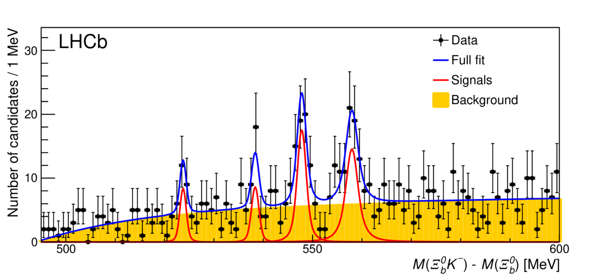
Four peaks are seen. The two higher-mass peaks are statistically very significant, and are incompatible with a background fluctuation. The two lower-mass peaks are also significant, but the possibility that they are due to a background fluctuation cannot be ruled out based upon this data sample. The absolute masses of these peaks — obtained by adding the known Ξb0 mass of 5792 MeV/c2 to the peak positions from the fit — range from 6315 – 6350 MeV/c2. It is also worth to point out the benefit of using the mass difference. While the mass resolution of the Ξb0 peak (see figure above) is approximately 15 MeV/c2, the mass resolution of these peaks is below 1 MeV/c2. As these peaks are the result of strong decays, the widths are due to a combination of each state’s natural width (usually a Breit-Wigner shape) and the detector resolution (Gaussian). These peaks represent the first observation of any excited Ωb– state.
More details, and additional measurements performed in the analysis can be found in the publication.
- Journal: Phys. Rev. Lett. 124, 082002 (2020)
- CERN Document System: LHCb-PAPER-2019-042