
LHCb is a general purpose experiment that specializes in the study of particles that contain beauty or charm quarks. A key feature of bb production at the LHC is the correlation between the angle of the b and b quarks in the proton-proton (pp) collision. The figure below shows the angle of the b quark versus the angle of the b quark in 7 TeV center-of-mass energy pp collisions. It shows that when one of the b-quarks has small angle, the other one usually does too. Or, if one b-quark has angle close to 180o, so does the other. Thus, if a detector is built to cover the forward region, say up to 350 mrad, one will capture a large fraction of events in which both the b and b are in the detector’s active region.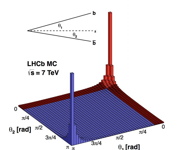
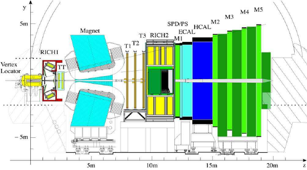
Thus, to maximize the physics potential of such an experiment, the LHCb detector is built in the “forward” direction, namely covering small angles with respect to the beamline. A cartoon of the LHCb detector is shown below.
One of the key reasons to capture both the decay products of both the b and b is to study CP violation. CP refers to the process of applying charge conjugation [1] and parity [2] to a given decay process. It is believed that precise studies of such phenomena can give insight into why the Universe is composed almost entirely of matter, and almost no antimatter. That is, even though it appears that the laws of physics (as we know them today) treat matter and antimatter about the same, the fact that the Universe has almost no antimatter contradicts this supposition. So, we are searching for phenomena where the matter and antimatter processes are unequal, and cannot be explained with the current theory of matter, the Standard Model.
Some of the measurements we perform, including CP violation, require us to identify whether a decaying b-hadron, say a neutral B meson, was a B0 or B0 meson when it was produced (at t = 0 sec after the pp collision). One interesting phenomena that requires this identification at t=0 is that of B0s mixing. In B0s mixing, a B0s meson (b s) can transform into a B0s (bs) meson through second-order weak processes involving virtual top quarks and W bosons. As a result, a particle that is produced as a B0s oscillates back and forth between being a B0s and a B0s meson as it travels, up to the point that it decays. The observable effect of Bs mixing is shown below, where the sample is separated into those Bs decays in which the B meson was produced as a Bs0, versus those produced as a B0s. In both cases, the Bs is detected through its decay to Ds–π+.
In principle, only a Bs can decay to Ds–π+, a Bs cannot. However, what can happen is a Bs can first transform into a Bs (through the second-order weak process mentioned above), and then it can decay into a Ds–π+. Thus, another way to interpret the data and curves below is that the blue points/curve represent unmixed decays and the red points/curve show when Bs mixing has occurred.
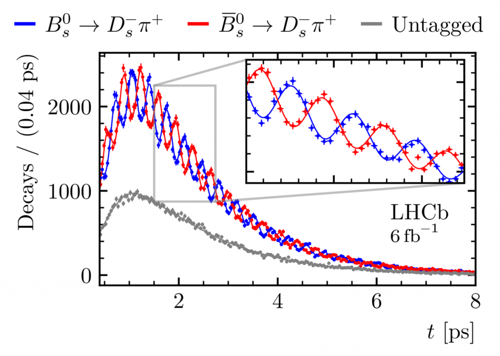
The observed decay time spectra shows oscillations in each sample, where the number of B0s mesons decrease and increase periodically, as do the number of B0s mesons. This is expected, because there are quantum processes that allow it to occur. The frequency of the oscillation, which is measured directly in such a measurement, depends on what kind of heavy particles are contributing to the matrix element of this process. Thus, by measuring the oscillation frequency in this spectrum, we are directly probing high mass particles that contribute to this process. If new physics particles can mediate the mixing, then they will likely modify the mixing frequency to be different than that expected in the Standard Model.
Turning to CP violation, we generally want to compare the decay rate (to a specific final state) of a particle decay with that of the CP conjugate decay. Let’s consider the “signal” decay we want to study to be B0 → J/ψK*0. In this case, one would like to compare the decay B0 → J/ψK*0 versus its CP-conjugate decay B0 → J/ψK*0 (the J/ψ is a cc state, and therefore is “self-conjugate”). The measurement requires one to know the “flavor” of the B at t = 0. Namely, was the B meson a B0 or a B0 at t = 0? Because B0 mesons (like Bs) can oscillate, even if you could determine the flavor when it decayed (based on the decay products seen), it does not tell you what the B flavor was at t=0! On the other hand, if one studies CP violation for a charged B decay e.g. B+(bu) vs B-(bu), then one is guaranteed that the flavor at decay is the same as at t=0. This is evident since the B+ cannot oscillate into a B-, as this would violate charge conservation.
Determining the flavor at the time of production is called flavor tagging. This is done using information from either (1) the other b hadron in the event (so-called “away-side tagging”), or (2) information on tracks produced in association with the signal B decay (so-called same-side tagging). The idea is illustrated in the figure below.
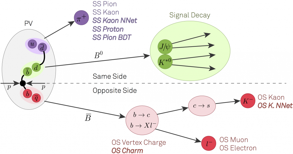
In opposite-side tagging, one looks to identify the flavor of the “other b hadron” in the event (here, a semileptonic B decay). This is because the beauty quarks are produced through the strong force, and the strong force always produces b and b. in pairs with opposite flavor. By examining the decay products of “the other b”, we can — with some probability of success — determine the flavor of the “other” b-hadron that produced the given decay products. Since the signal b-hadron must have the opposite flavor, this tells us the flavor of the signal B hadron. In the cartoon above, if we detect a high transverse momentum μ– lepton that does not come from the pp collision point, there is a high probability it is associated with a semileptonic b decay. Thus, the signal b-hadron must have contained a b quark in it at t = 0. Conversely, if one observed a high transverse momentum μ+ lepton that does not come from the pp collision point, it likely comes from a semileptonic b decay, and thus the signal b-hadron contained a b quark at t = 0. Other decay products can be used as well, e.g. any charged kaons or electrons from the other b hadron. ,One can also use more sophisticated combinations of particles, such as forming a displaced vertex and use the total charge of the tracks used to form the vertex. Since a b quark has charge -1/3 and a b has charge +1/3, one would expect the “vertex charge” to preferentially be negative for b quarks and positive for b quarks. One can also look to reconstruct various charm mesons, and their identity is a powerful means with which to flavor tag.
Same-side tagging uses particles that are produced close in space (e.g. transverse momentum and pseudorapidity) to tag the flavor of the signal b-hadron directly. This is most effective for tagging Bs mesons. The logic here is as follows. In the pp collision, suppose the signal Bs meson contained a b quark. To make a Bs meson, the b quark needs to bind with an s quark. The strong interaction produces strange quarks in pairs, e.g. ss. In this case, if the b quark binds with an s to form the Bs meson, there is a s quark “left over”. This s quark must also form a hadron. If it forms a kaon, it has to be either K0(sd) or K–(su). In the latter case, the observed K– would tell us that the Bs meson must have contained a b-quark at t=0 (it was a B0s at t=0). Conversely, if we were to find a same-side K+ meson, it would tell us that the Bs meson contained a b quark at t = 0 (it was a B0s at t = 0).
None of these tagging methods get the flavor correct all of the time, and in fact each tagging method’s effectiveness needs to be measured using data. There are a host of ways to do this, which are documented in on this LHCb flavor-tagging publications page. Briefly, for any given flavor-tagging algorithm, we need to quantify its efficiency and the dilution. The efficiency is how often the algorithm provides a flavor tag, e.g. ε = Ntag/Nsignal; it matters not whether the tag is correct or not, just the algorithm made a decision. The dilution, D gives the fraction of time that you get the correct flavor, and is defined as: D = (Nright – Nwrong) / (Nright + Nwrong). The effective flavor-tagging efficiency is given by εeff = εD2. If either ε = 0 or D = 0, you have not ability to flavor tag. If D=0 for your flavor tagging algorithm, it gets the b-quark flavor right as often as it gets it wrong. That is, you may as well be flipping a coin… so back to work on it! So, to have any chance at flavor-tagging, your algorithm/scheme must get the flavor right more often than wrong (D > 0).
One can improve the overall flavor tagging by using all algorithms together, and accounting for their correlations. At the end of the day, in LHCb, we obtain an effective flavor tagging efficiency εeff ~ (6-8)%, where the value depends on the specific signal decay.
So far, we have discussed mainly B0 and Bs, both of which are beauty mesons. But, in general, many different kinds of beauty hadrons can form in proton-proton collisions at the LHC. While it is beauty quarks that are produced in the pp collision, the strong interaction soonafter takes hold, and stable beauty hadrons form in a very short time scale, of order 10-23 sec. It is these beauty hadrons that we observe. In particular, a b quark can combine with any other antiquark (except the top quark [3]) to form a B meson. Similarly, a b-quark can combine with two other quarks to form a beauty baryon (again, excluding the top quark). Thus one could have quite a large number of possible baryons! Most recently, there are strong indications of four and five-quark objects as well.
Although many types of beauty hadrons can be produced, they are not all produced with equal probability. To know how many b-hadrons of a specific type we produce, we can rely on the following formula, where we’ll use the Bs meson as an example.
N(Bs→mode) = 2 σ(pp → bb) fBs Lint B(Bs → mode) Acc(LHCb) ε(mode)
Here, σ(pp → bb) is the cross-section for producing bb in pp collisions at a given center-of-mass energy in [barnes] [4], fBs is the fraction of the time that a b-quark fragments into a Bs meson, Lint is the integrated luminosity in [barnes]-1, B(Bs → mode) is the branching ratio for the mode in which the decay is being detected, Acc(LHCb) is the probability that at least one Bs is within the LHCb detector acceptance, and ε(mode) is the efficiency for detecting the chosen Bs decay mode. The factor of 2 is because beauty quarks are almost always produced in pairs. The fragmentation fractions express the probability that a b-quark fragments into a particular b-hadron, and in general these fractions have to be measured. Morever, they may depend on the environment that they are produced (e.g. e+e– vs pp collisions) and/or on the kinematics (transverse momentum and rapidity).
Because the processes under study are not so abundant, they are often measured in [ub] = 10-6 [barn], or even [nb], or [pb]. On the other hand, integrated luminosity is frequently given (at the LHC) in [fb]-1. This is convenient, since multiplying σ(pp → bb)× fBs × Lint gives you the number of Bs mesons produced for a given integrated luminosity. So, if σ(pp → bb)~300 ub, fBs ~ 0.1, and Lint = 5 [fb-1], and Acc(LHCb)~28%, that implies that about 42 billion Bs are produced within the LHCb acceptance. Since B(Bs → mode) can range from 10-2 (mode = Ds–π+) to 10-9 (μ+μ–), one can end up with samples of millions of reconstructed decays, or as few as just a handful.
The qualities that makes LHCb unique in b-hadron physics include
-
Detection of both b and b-bar quark to allow for CP violation measurements
-
All species of b-hadrons are produced.
-
Beauty hadrons tend to have large momentum along the beam axis, so weakly-decaying beauty hadrons travel several mm’s (or even cm’s) before decaying.
-
The LHCb detector includes devices (RICH detectors) to distinguish protons, kaons and pions.
-
Very flexible trigger system to select events of interest, and toss away the uninteresting events. Also, large event rate to tape possible (~10 kHz in Run 2).
Because all species of b-hadrons are produced, one can not only look for the weakly-decaying beauty hadrons, but one can look for strong decays of excited b-hadrons, that decay to the ground state. A classic example, is the excited Λb states, Λb(5912) and Λb(5920), both which decay to Λbπ+π–. Here, one reconstructs the weakly-decaying Λb (typically through its decay to Λc+π–), and then one pairs this reconstructed Λb with a π+π– pair from the pp collision point. Significant peaks are seen in the invariant mass spectrum of the Λbπ+π– candidates, as shown below (from LHCb-PAPER-2019-045).
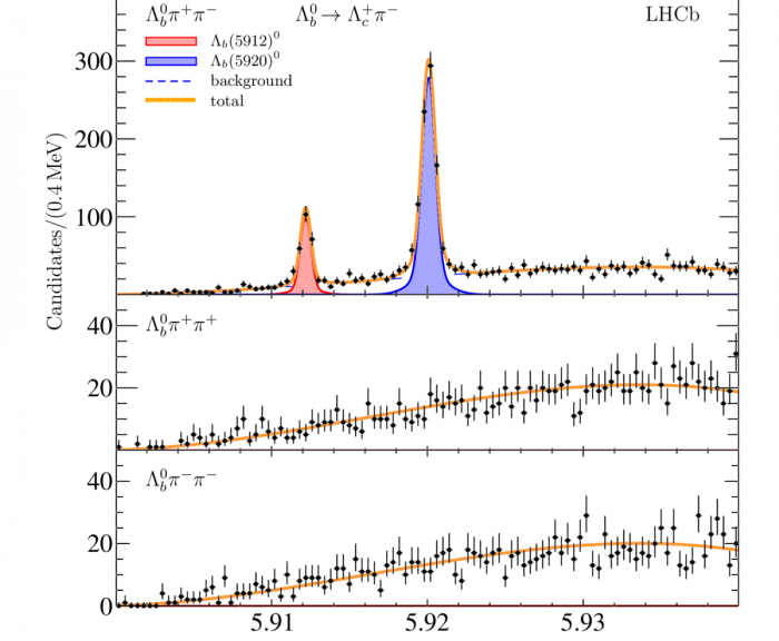 As the plot shows, only when you combine the Λb with oppositely-charged pions, you see the peaks. No peaks are seen when combining with same-sign pions, as there is no such decay expected with same-sign pions.
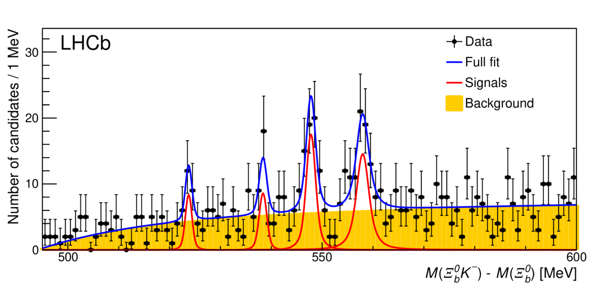
Or, in a similar way, one combines a fully-reconstructed Ξb0 with a K–, and finding the Ξb0K– invariant mass spectrum below (see LHCb-PAPER-2019-042).
Many such analyses have been carried out in LHCb, where one combines a ground state beauty hadron with 1 pion, 2 pions, one kaon, a kaon plus a pion, and so on. This has led to observations of many of the excited beauty meson and excited baryon states, and there are more discoveries to come.
There are numerous possibilities for studying the physics of beauty and charm hadrons in LHCb, as well as other areas such as heavy ion collisions, Electroweak investigations (W, Z and top quark), studies of exotic hadrons (those containing something other than qq or qqq), and so on.
A full list of LHCb publications can be found here.